4. Resampling
In data integration, resampling of images is an important pre-processing step, especially when we are dealing with datasets with different spatial resolutions and scales. When the differences in the spatial resolution between the input and the output are small, simple interpolation methods are good enough for estimating pixel values. However, when such differences are significant, then we need to apply aggregation.
The image you will be working on is a subset taken from band 1 of Landsat 5 sensor, and it has a pixel size of \(30 \ m\).
Important
Resources. You will require the latest LTR version of QGIS (A Coruna 3.10), plus the dataset resampling.zip which you can download from CANVAS. When you unzip the dataset, you will find the following files inside:
l5_20100627_band1.tif- an image subset from band 1 of Landsat 5 and spatial resolution of \(30 \ m\).grid.shp- a vector dataset representing a grid for the original pixel size of the Landsat 5 image.average.txt- a file with a kernel filter definition.Resampling.qgs- a QGIS project file loaded with data layers and styles.
- Task 1
Make sure you have the Map swipe tool and Value Tool plugins installed.
- Task 2
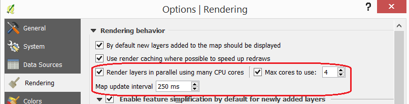
Configure QGIS to render layers using multiple CPU cores. Go to Settings > Options > Rendering and make sure the option Render Layers in parallel using many CPU cores in on. Set Max Cores to the number of CPU cores in your computer, use at least 4 for better performance. See below.
4.1. Basic Resampling
Assume that we are going to use the Landsat image as input for a model. The model requires a grid size of \(50 \ m\). Thus we have to resample the image to a pixel size of \(50 \ m\) before proceeding with the modelling.
Note
Reflection. In this section, we make the assumption that applying a resampling before the primary data processing operations (modelling in this case) is the correct procedure. Note that in many cases it may be more accurate to process the image first and then do the resampling.
Read the details about resampling on the  Geocoding page.
4.1.1. Resampling Techniques
- Task 3
Start QGIS and open the ‘Resampling’ project. From the Processing toolbox, open the tool r.resamp.interp and resample the image
l5_20100627_band1.tifto \(50 \ m\). Use the nearest (neighbour) interpolation method. See Fig. 4.8 Provide a self-descriptive name for the output file, for example: nearest_50
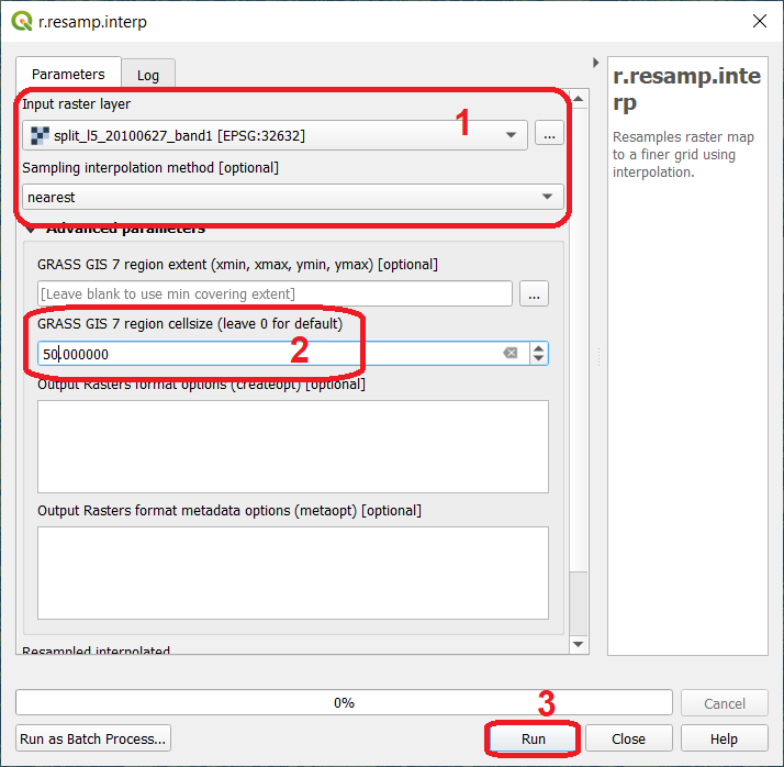
Fig. 4.8 The ‘r.resamp.interp tool. Resampling to 50 m using the ‘nearest’ method
- Task 4
Repeat the previous task. This time use the bilinear and bicubic interpolation methods. Make sure to provide meaningful names for the outputs. For example: bilinear_50, and bicubic_50 respectively.
Attention
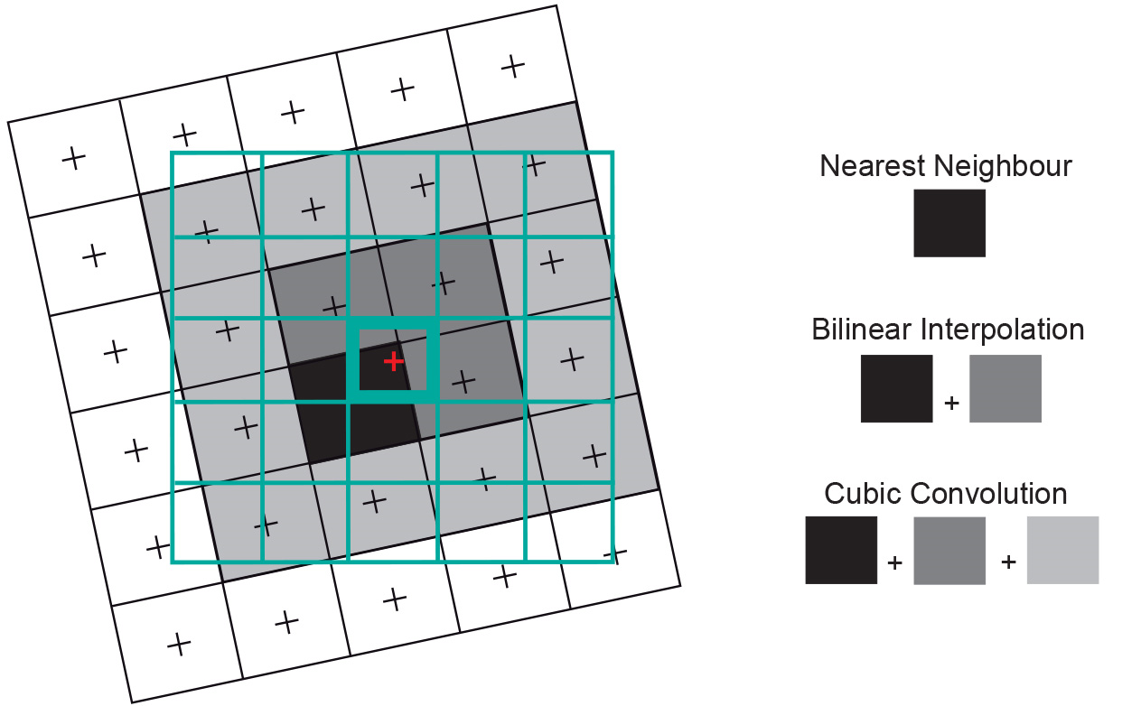
Question. Resampling relies on interpolation techniques, and therefore it depends on Tobler’s first law of geography: locations that are closer together are more likely to have similar values than locations that are farther apart.
Keeping that law in mind and look at the image below. It shows (for the pixel marked in red) which neighbouring pixels are considered in every interpolation technique.
Can you think of a use case where one resampling techniques should be prefered over the others? Why?
- Task 5
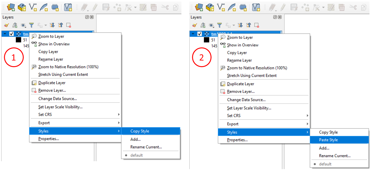
Copy the style of layer ‘l5_20100627_band1’ and paste it on the resampled layers you created. To copy the style: Right click on ‘l5_20100627_band1’ > Styles > Copy style. See below. To paste the style: Right click on the layer where your want to paste the style > Styles > Paste style.
Having the original and the resampled images with the same style will make it easier to compare the result of the different resampling techniques.
4.1.2. Comparing the Results
You should now have four raster layers in your project. The original Landsat band 1 and three additional images; the results from the resampling. See Fig. 4.9
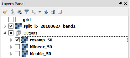
Fig. 4.9 Layers resulting from the resampling of ‘l5_20100627_band1’ using different techniques
Note
Reflection. When resampling is applied to an image to produce a version with lower resolution, no new radiometric information is produced. That is resampling changes the pixel size, but it does not produce further information. On the contrary, resampling often implies a loss of information, and in the case of lower resolution a loss of spatial precision. Despite that, resampling is a technique that is required in many cases to integrated datasets with different spatial resolution. What should be carefully considered is if the loss of information and precision are acceptable for the analysis or not.
- Task 6
Perform a visual comparison of the size and values of the pixels of the four raster layers. Zoom into to ‘grid’ layer and explore the raster layers using the Value tool and Swipe map tool plugins. Watch the video tutorial on visually comparing rasters.
Note
Reflection.
Relate the differences you observe in resampled layers with the theory you learned in resampling and Geocoding.
Another way to compare the resampling results is by using a histogram. A histogram will show the differences in the distribution of the values. To do this, we need to stack the individual resampling results in a single layer stack.
- Task 7
From the Processing Toolbox, open the Build Virtual Raster tool. For Input layers select: ‘l5_20100627_band1’, ‘nearest_50’, ‘bilinear_50’ and ‘bicubic_50’. Name the resulting stack as stack_50. See Fig. 4.10
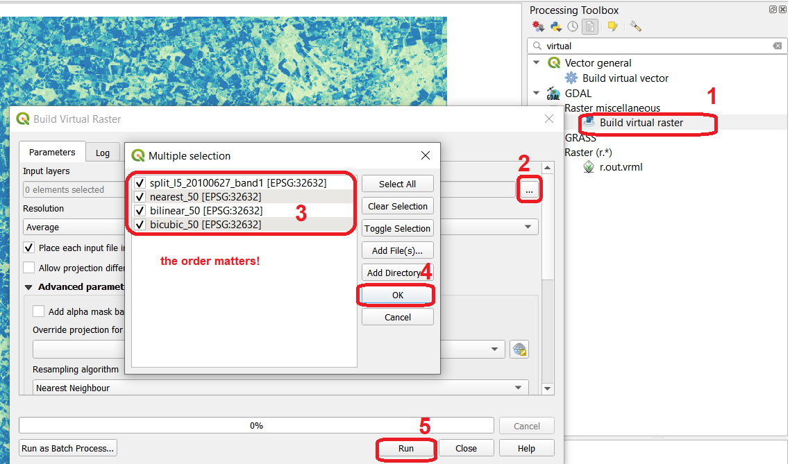
Fig. 4.10 Building a virtual raster stack with the resampled raster layers
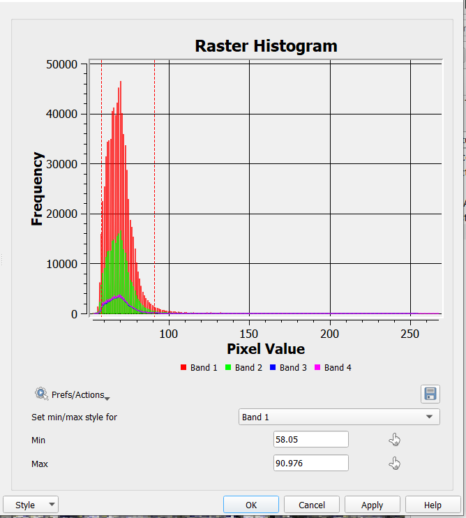
- Task 8
Compute the histogram for all bands of the ‘stack_50’ stack. Right click over ‘stack_50’ layer > Properties > Histogram > Compute histogram. You should see a histogram like the one below:
Attention
Question. How do you explain the differences in the distribution of values in the histogram? Especially for band 2 (nearest_50) and band 4 (bicubic_50).
4.2. Advanced Resampling
For many practical applications, you have to resample an image to much larger pixel sizes than the original. In this section, you will resample the image to a pixel size of \(200 \ m\). For the sake of comparison, you will use an optimal and a sub-optimal method.
4.2.1. Optimal Resampling: with Aggregation
Resampling an image to a relatively larger pixel size means that the radiation values, in the original image, must be integrated from a much larger surface area than the original. That is, for this case, to integrate the radiation values from an area of \(30 \ m \times 30 \ m\) to an area of \(200 \ m \times 200 \ m\). To do so, we first have to do an aggregation (i.e. a convolution filter) and do the resampling only after that.
- Task 9
From the Processing toolbox, open the tool r.mfilter and apply a low-pass kernel of \(7x7\). Such kernel will average the data over a 7 by 7 pixels area, that is \(30 \times 7 = 210 \ m\). Therefore, the kernel filter aggregate the radiation value for an area of \(210 \ m\) by \(210 \ m\).
As Input layer choose ‘l5_20100627_band1’ > for Filter file use the
average.txt> for Filtered typeaverage_7x7.tif> Run. See Fig. 4.11
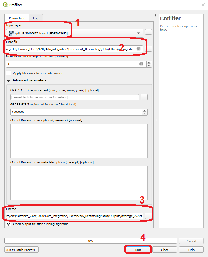
Fig. 4.11 Aggregation of radiation values using the ‘r.mfiltr’ tool
- Task 10
Use the r.resamp.interp tool and resample the
average_7x7.tifto a pixel size of \(200 \ m\). Use the nearest interpolation method. Refer to Task 3 if you need to.
4.2.2. Sub-Optimal Resampling: no Aggregation
To understand the reason why we should aggregate prior a resampling when the resampling resolution is much larger than the original pixel size. Now, you will apply only a resampling of \(200 \ m\) to the Lansat image.
- Task 11
Use the r.resamp.interp just like you did in the previous tasks. Use the ‘l5_20100627_band1’ as input layer, nearest as interpolation method, and \(200 \ m\) for pixel size.
4.2.3. Comparing Optima and Sub-Optimal Results
- Task 12
Compare the resampled layers with and without aggregation. Use the technique you used in Task 6.
- Task 13
Plot the histograms for the resampled layers with and without aggregation. If necessary, save the histogram(s) to a file so that you can look at both of them at the same time.
Attention
Question.
When comparing the resampled images with and without aggregation. Which one shows a ‘smoother’ image? Why?
Which resampled images has a smaller value range? Why?
Section author: Zoltán Vekerdy, André Mano & Manuel Garcia Alvarez