3. Digital Image Classification
In this exercise, we use a Sentinel-2 satellite image covering Enschede and its surroundings from September, 2016. Before going forward with the exercise read about  digital image classification.
Important
Resources. You will require the latest LTR version of QGIS (A Coruna 3.10), plus the dataset digital_image_classification.zip which you can download from CANVAS. When you unzip the dataset, you will find the following files inside:
s2_25_sept_2016.tif, a Sentinel-2 satellite image of Enschede.Training_areas.shp, containing the sites visited during a fieldwork.digital_image_classification.qgs, a project containing the files above.Field_Photos_201, a folder containing photos of the surroundings of training areas.
The methodology for mapping land cover using satellite images consist of the following general steps:
Interpretation of satellite image
Field data collection
Field data analysis
Supervised Classification
Accuracy assessment
In this exercise, you will conduct the steps mentioned above except for the Field data collection. However, we briefly explain that step in the sections Field Survey and Organising Field data. The workflow in Fig. 3.2 summarized the process of applying digitial image classification for land cover mapping.
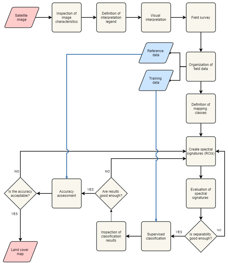
Fig. 3.2 A workflow of the process of digital image classification for land cover mapping
3.1. Inspection of Image characteristics
The first step is to get familiar with the dataset by reviewing the characteristics of the image dataset. We will use only some of the spectral bands of the Sentinel image because of their differences in spatial resolution.
- Task 1
Inpect Table 3.1., open
s2_25_sept_2016.tifin QGIS and get familiar with this dataset. Notice that the bands in the image refer to the numbers under the column Exercise Band.
Band |
Wavelength (\(\mu m\)) |
Bandwith (\(\mu m\)) |
Resolution (\(m\)) |
Exercise Band |
|---|---|---|---|---|
Band 1 (VIS) |
0,443 |
0,02 |
60 |
\(-\) |
Band 2 (VIS) |
0,49 |
0,065 |
10 |
1 |
Band 3 (VIS) |
0,56 |
0,035 |
10 |
2 |
Band 4 (VIS) |
0,665 |
0,03 |
10 |
3 |
Band 5 (RE) |
0,705 |
0,015 |
20 |
4 |
Band 6 (RE) |
0,74 |
0,015 |
20 |
5 |
Band 7 (RE) |
0,775 |
0,02 |
20 |
6 |
Band 8 (NIR) |
0,842 |
0,115 |
10 |
7 |
Band 8A (NIR) |
0,865 |
0,02 |
20 |
\(-\) |
Band 9 (NIR) |
0,94 |
0,02 |
60 |
\(-\) |
Band 10 (SWIR) |
1,375 |
0,02 |
60 |
\(-\) |
Band 11 (SWIR) |
1,61 |
0,09 |
20 |
8 |
Band 12 (SWIR) |
2,19 |
0,18 |
20 |
9 |
3.2. Legend & Visual Interpretation
The interpretation process involves to visually examine the image dataset that will be use in the classification, and define a set of classes of interest. In this case we will focus on the definition of classes of land cover. For example, forest, buil-up areas, water bodies, grass fields, etc.
3.2.1. Interpretation Legend
The interpretation legend defines a list of legend units in terms of the characteristics of the image dataset. For example, one unit can be define as all black and dark-blue pixels in the image.
- Task 2
Start QGIS and open the
s2_25_sept_2016.tif, display it with the band combination 7,8,3.Define between 5 to 10 legend units for this dataset. After we established a legend, we can start with the visual interpretation.
3.2.2. Visual Interpretation
One the purposes of Visual image interpretation is to identify objects in the image dataset. For this we use the legen units defined in above and the ability of the human eye to recognize certain objects. For example, a legend unit defined as black and dark-blue pixels can be recognized, after considering the size, shape and texture of the objects , as water.
Attention
Question. Base on your knowledge on the image characteristics and EM radiation, which classes of land cover can you name and identify?. If your now sure use the QuickMapService to load the standard map from Open Street Maps.
3.3. Field Survey
The purpose of the fiel survey or fieldwork is to conduct a survey to determine what the legend units based on theimage characteristics are in reality. In this case, what type of land cover and land use they represent.
During the survey we have to visit and check different locations for all the legend units. Then, we record our observations at each location. The locations for the survey should be chosen in such a way that all legend units are covered.
In this course, it is not possible to conduct a fieldwork. Instead, we provide you with a dataset with observations made during a fieldwork for interpreting the Sentinel-II image in Enschede, NL. The datasets contains locations and photos for each visited site. If you were to conduct a field surves, you should collect similar data.
- Task 3
Add the
training_areas.shpto QGIS. Use the Identify tool to inspect the location of visited sites during the fieldwork over the ‘s2_25_sept_2016’ image. Put attention to the attributes TA_ID, it tells the file name of the photo(s) that belong to that location; for example. AV_1. If more than one photo is available for a location, files names contain also a literal; for example AV_1a and AV_1b. See Fig. 3.3
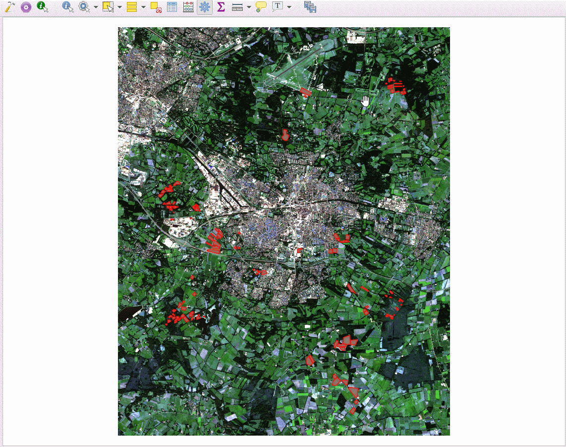
Fig. 3.3 Field data: training data and photos.
3.4. Organising Field data
After fieldwork, we have to structure the fieldwork data, define classes and relate such classes to the image. Thus we have to define field classes using the fieldwork data. Filed classes are classes recognizable in the field based on certain criteria. In our case the creteria is related to land cover and land use. Field classes should define at same level of detail.
- Task 4
Compare the field classes, as defined in the attribute Landcvr of the ‘training_areas’ layer, with the colours on the satellite image when displaying bands 7,8,3. Make a list of up to 10 map classes you would like to classify, and write down which colour(s) corresponds them. See the example in the table below.
Class
Colour (7-8-3)
Water
Black/dark blue
3.5. Defining Mapping Classes
In the previous task, you practiced how to define field classes and associate colours. However, for the remainder of this exercise, we will use the following list of macroclasses (MC_info) and ID codes (MC_ID).
MC_ID |
MC_Info |
|---|---|
1 |
water |
2 |
maize |
3 |
evergreen |
4 |
grass |
5 |
bare |
6 |
buildings |
7 |
tarmac |
8 |
heath |
9 |
deciduous |
10 |
rapeseed |
It is fundamental that you follow the nomenclature above, because the accuracy assessment assumes that the classification results contain such classes.
3.6. Defining Spectral Signatures (ROIs)
Note
QGIS. The QGIS Semi-automatic Classification plugin uses the term ‘Region of Interest’ (ROI) instead of ‘training sample’ which is the term you will see in the reading materials. These terms are equivalent and have exactly the same meaning.
- Task 5
Install the plugin Semi-automatic classification. If necessary, open the
s2_25_sept_2016.tif.- Task 6
Use the Semi-automatic classification plugin to create the first training sample. While you are at it, follow these recommendations:
Make sure that you take samples from homogenous areas, and that the standard deviation is kept low (check the statistics of the ROI).
It is advisable to make several subclasses for the same macroclass. For example, you will notice that not all pixels with water have exactly the same colour. Some areas with water have black pixels and some others have dark-blue pixels. Instead of collecting samples under the macroclass water, it is better to split water in two subclases, for examples water_black and water_blue, and take samples for each subclass separatly. The set of all pixels associated to an specific class is what we call a spectral signature.
Give subclases distinct class names (e.g. grass_yellow, grass_orange).
Watch the video tutorial on Creating training sets to know how to complete this task in QGIS.
Note
QGIS. We will apply a classification based on macroclasses (information class), and not on subclasses (spectral classes). When we classify according to macroclasses, the classification algorithm will group subclasses and label the results according to macroclass. However, the classification algorithm will not merge the spectral signatures.
Attention
Question. Why is it advisable to make separted (spectral) subclasses when taking training samples?
- Task 7
Define ROIs for all macroclasses in the table above and for all relevant subclases. Remember to group subclases with the correct macroclass.
3.7. Evaluation of Spectral Signatures
You can visualise spectral signatures (ROI) statistics. One option to evaluate signatures (ROI) are feature space images , which are two-dimensional histograms.
- Task 8
Create and analyze feature spaces. Click on Add highlighted items to scatterplot as shown in minute 11:15 onwards of the video tutorial on Creating training sets. Insepect the feature spaces and evaluate the separability of your ROIs.
Attention
Question. What band combination creates a suitable feature space to evaluate the separability of your training samples?
To evaluate the quality of the training samples, we can the standard deviation as reference.
- Task 9
Analyse the standard deviation for each of your ROI. Click on Add highlighted signatures to spectral signature plot > Signature details.
When you are satisfied with the signatures (ROI) of your training samples, you can move to perfom a digital image classification.
3.8. Supervised Image Classification
In this exercise, we will use the Maximum Likelihood classifier for the supervised classification, but we encourage you to experiment with other classifiers and compare the results.
- Task 10
Use the Semi-automatic classification plugin to test your first training sample set. Configure the ‘Classification algorithm’ as shown in Fig. 3.4. Then use the Active classification preview pointer
 to generate a temporary classification. Then, visually inspect the classification results.
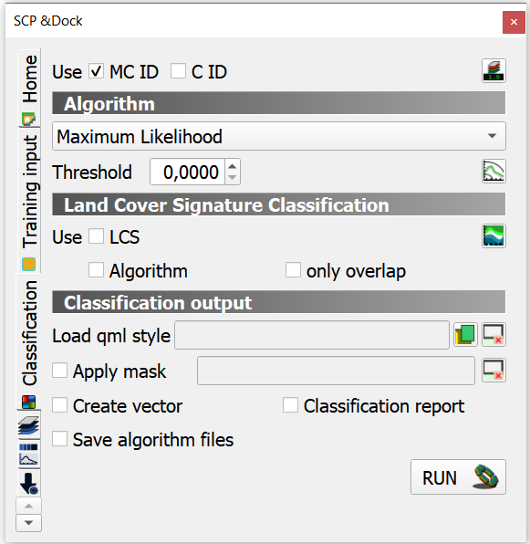
Fig. 3.4 Setting a classifier
Watch the video tutorial on Running a supervised classification to complete this task.
3.8.1. Inspect Results & Improve the Classification
- Task 11
Based on the visual inspection of your first classification results, add additional ROIs that capture areas where the algorithm fails to classify the image correctly.
Then, inspect the classification results again, and if necessary add more ROIs until you are satisfied with the results.
- Task 12
Run the final classification, by clicking on the button
- Task 13
Generate a shapefile from the ROIs you used to classify the image. [HOW? GIVE SOME HINT?]
- Task 14
Make sure you save your training samples for later use. In the Semi-automatic classification plugin, this is done automatically.
3.9. Accuracy assessment
Important
Resources. In this section, you will will require the dataset reference_data.zip, which you can download from CANVAS. This dataset contains the following file:
reference_data.shp, dataset containing the locations and types of land cover for the accuracy assessment.
3.9.1. Data for Accuracy Assessment
For this exercise, the data for the accuracy assessment have been collected for you. The reference_data.shp contains the ground truth information of 187 locations, that we will use in assessing the accuracy of the supervised classification.
The areas in the reference_data.shp were randomly selected. Areas which fell on the edge of two or more classes were considered.
- Task 15
Add reference_data.shp to QGIS and open its attribute table. Make sure the values for MC_ID and MC_Info attributes match the ones you used for the macroclasses during the supervied classification of the ‘s2_25_sept_2016’ image.
3.9.2. Accuracy Report
In the accuracy assessment, we generate an Error matrix between the classification results and the reference data. The accuracy report will provide the overall accuracy of the classification, as well as user and producer accuracies.
- Task 16
Perform the accuracy assessment. Watch the video tutorial on Accuracy assessment of supervised classuification.
3.9.3. Improve Accuracy
The accuracy of the classification can be improved by identifying the sources of errors in the process of supervised classification, and then minizing their effects on the classification results.
- Task 17
Locate and inspect areas which you suspect are soruces in your classification result. Then, try to improve the overal accuracy by adding or excluding ROIs from your training dataset.
Once the accuracy of the supervised classification is acceptable, you have completed the digital image classification process and generated a land cover map. Save all your results.
Attention
Question. What determines if the accuracy of the digital image classification is acceptable or not?
Important
Assignment Submission
Read the instructions of the Digital Image Classification Assignment, and submit your results before 7th October 23:59 (GMT+2).
Section author: Monika Kuffer, Andre Mano & Manuel Garcia Alvarez