5. Mono and Multi-Temporal Classification
In section Digital Image Classification, we apply image classification to classify land cover, to a dataset containing images for a single date (mono-temporal). However, no all classes of land cover are equally distinguishable any time of the year. For example, seasonal crops like maize can only be distinguished during their growing season. Some types of trees (e.g., deciduous trees) change their spectral reflectance thru the year, because of changes in their foliage. In such cases, we can use images from multiple dates ( multi-temporal) to increase the level of information in the classification process.
In this exercise, we demonstrate the advantage of using multi-temporal data in image classification, to increase the separability between classes. We use the case of land cover mapping as an example.
Important
Resources. You will require the latest LTR version of QGIS (A Coruna 3.10), plus the dataset mono_bi_temporal_classification.zip which you can download from CANVAS. When you unzip the dataset, you will find the following directories and files:
Landsat - Images from the Lansat-TM, from 2010-06-23:
L5197024_02420100627_B10.tifL5197024_02420100627_B20.tifL5197024_02420100627_B30.tifL5197024_02420100627_B40.tifL5197024_02420100627_B50.tifL5197024_02420100627_B60.tifL5197024_02420100627_B70.tif
ASTER - Images from the ASTER, from 2010-04–23:
VNIR_Swath_1.tifVNIR_Swath_2.tifVNIR_Swath_3B.tifVNIR_Swath_3N.tifSWIR_Swath_4.tifSWIR_Swath_5.tifSWIR_Swath_6.tifSWIR_Swath_7.tifSWIR_Swath_8.tifSWIR_Swath_9.tifTIR_Swath_10.tifTIR_Swath_11.tifTIR_Swath_12.tifTIR_Swath_13.tifTIR_Swath_14.tif
Shapefiles:
Evaluation.shp- areas with three distinct land cover classes.AreaOfInterest.shp- spatial extent for band subsets.
Output: - An empty directory to store your results.
mono_bi-temporal_classification.qgs- a QGIS project loaded with the files listed above.
5.1. Setting Up the Analysis Environment
Before starting with the processing and analysis of the data in this exercise, we need to add specific tools for remote sensing to QGIS.
- Task 1
Make sure that the Semi-automatic Classification (SCP) and Value tool plugins are installed.
- Task 2
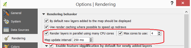
Configure QGIS to render layers using multiple CPU cores. Go to Settings > Options > Rendering and make sure the option Render Layers in parallel using many CPU cores in on. Set Max Cores to the number of CPU cores in your computer, use at least 4 for better performance. See below.
In the following sections, we will conduct data analysis to compare the differences between mono-temporal and bi-temporal digital image classifications. The workflow in Fig. 5.6 shows the steps (operations) for such data analysis.
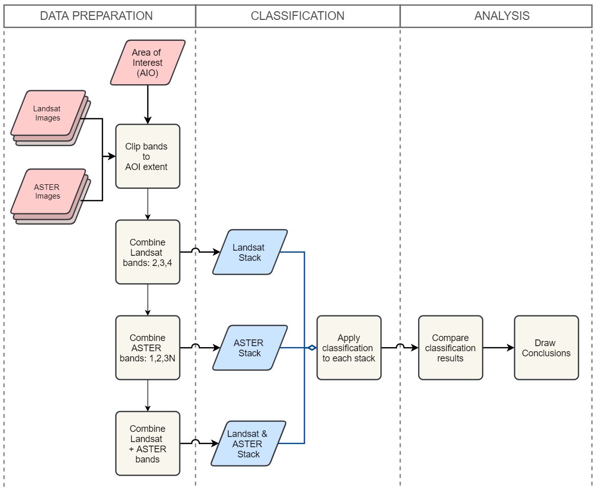
Fig. 5.6 A flowchart for the comparison of ‘mono’ and ‘bi’ temporal image classification
5.2. Data Preparation
5.2.1. Band Subsetting
You will start by stacking bands in three different combinations. One stack will combine three bands from Landsat-TM from the 23-Apr-2010. Another stack will combine three bands from ASTER, taken on the 23-Jun-2010. Finally, the last stack will combine all the bands in the previous two stacks: three Landsat bands and three ASTER bands.
- Task 3
Start by learning about the characteristics of the Landsat TM and the ASTER sensors. Put special attention to the wavelengths of the different bands. Note that the SWIR bands are not available in the ASTER images since 2008 due to the deterioration of the cooling system of the sensor.
Use the ITC Sensor Repository for this task:
Attention
Question. Which three bands of Landsat TM and ASTER are very similar?
Now that you known which bands are are identical. We will create a subset for the area in the AreaOfInteres.shp. That is, we will clip each band to the extent of the polygon in such file.
- Task 4
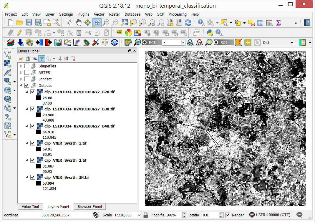
Open the QGIS project
mono_bi-temporal_classification.qgs. Go to SCP > Band set. Many of the operation available in SCP required to define a band set in advance. Then, the operation will be applied to all the bands in a set. SCP uses numbers to differentiate between band set. The current project already contains a band set (1) listing the all the bands we will need in this exercise. See Fig. 5.7
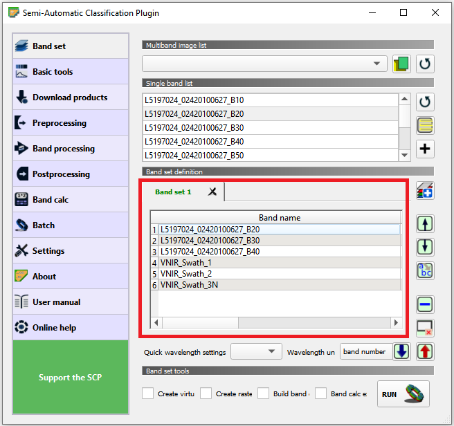
Fig. 5.7 Band set 1 in the ‘mono_bi_temporal_classification’ project
Go to Preprocessing > Clip multiple rasters. For Select input band set select 1. Then, make sure the Output name prefix is set to
clip. Tick Use shapefile for clipping and select the ‘AreaOfInterest’ layer. See Fig. 5.8 Finally, click on.
The tool will ask you to provide a directory to store the output files. For convenience, use the empty Output folder inside root directory for this exercise.
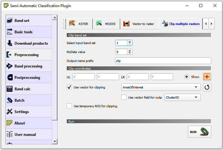
Fig. 5.8 The ‘Clip multiple rasters’ tool in the SCP plugin
Note
Reflection. Keep your QGIS project organised. The ‘mono_bi-temporal_classification’ project has a layer group named “Outputs”. Place the outputs of this exercise under this group. Alternatively, you can create more groups to keep the project even more organised.
Moreover, avoid having all the layers turned on. Especially the original Landsat and ASTER layers; they will consume resources every time you zoom or pan over the map view.
5.2.2. Band Stacking
As a next step, you will create three band stacks using the subsets created above:
The first stack with Landsat bands \(2, 3\) and \(4\)
The second stack with ASTER bands \(1, 2\) and \(3N\)
The third stack, a multi-spectral and multi-temporal stack with Landsat bands \(2, 3, 4\) and ASTER bands \(1, 2, 3N\)
- Task 5
Create a new band stack for Lansat. Go to SCP > Band set. Then Add a new band set > Select bands \(2,3,4\) from Landsat (clip version) > Add band to Band set > check that bands are in the correct oder > tick Create raster or band set > Run. See Fig. 5.9. Save the stack to the Output directory.
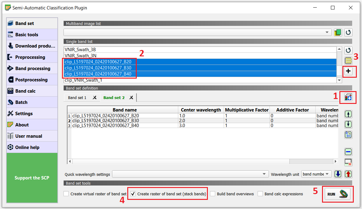
Fig. 5.9 Creating a new band stack in the SCP plugin
Note
QGIS. The QGIS does not preserve the original numbering of the bands in the new stack. This means you have to keep track of which bands in the new stack correspond to the original dataset.
For the stack you just created, that means:
Original band number (Landsat) |
Band number (New Stack) |
|---|---|
2 |
1 |
3 |
2 |
4 |
3 |
You can verify the new stack combined the correct bands and in the right order, using the Value tool plugin.
- Task 6
Open the Value Tool panel. Go to View > Panels > tick the Value Tool. Enable the panel; make sure only active layers are the three Landsat subsets and the new stack. Hover your mouse over the image and check that the pixel values correspond between the subsets and the new stack. See Fig. 5.10
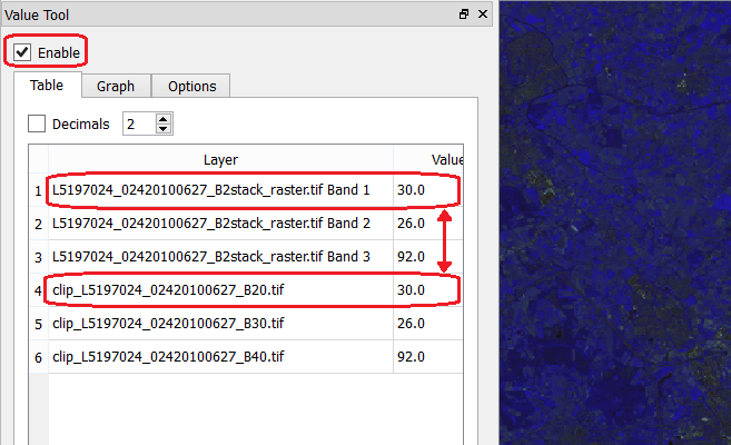
Fig. 5.10 Comparing pixel values between the ‘Lansat subsets’ and the ‘Landsat 2,3,4 stack’.
- Task 7
Repeat the procedure in the previous Task, and create two more stacks. One for ASTER bands \(1, 2, 3N\). And one for the ‘multi-spectral and multi-temporal’, bands Landsat \(2, 3, 4\) and ASTER \(1, 2, 3N\) Remember to keep track of the order of the bands in the stacks. We suggest the following arrangement:
For ASTER band stack
Original band number (ASTER)
Band number (ASTER stack)
1
1
2
2
3N
3
For Multi-spectral and Multi-temporal stack
Original band number (ASTER)
Band number in Stack
Landsat 2
1
Landsat 3
2
Landsat 4
3
ASTER 1
4
ASTER 2
5
ASTER 3N
6
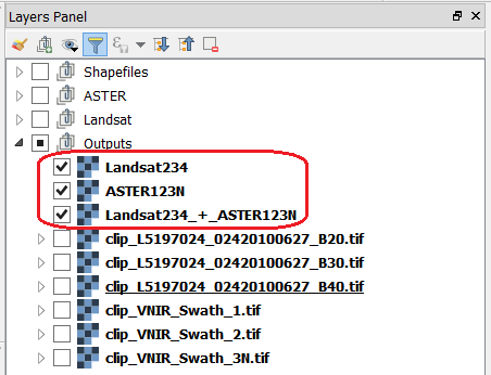
Now, you should have three band stacks in your project. We recommend you rename the stacks in the Layer panel so that you can easily distinguish them. See below.
5.3. Classification
Next, you will perform unsupervised classification using the band stacks you created. We will use a k-means clustering algorithm to identify different classes of land cover. For the sake of simplicity, we will name each class of land cover using numbers.
You will apply unsupervised classification to each band stack: Landsat stack, ASTER stack, and m*ulti-spectral and multi-temporal stack*.
- Task 8
Unclutter your project by removing the layers you will not need anymore. Remove the groups ‘Landsat’ and ‘ASTER’; keep only the shapefiles and the band stacks.
- Task 9
From the Processing toolbox, open the tool K-means clustering for grids, and provide the following parameters (Fig. 5.11):
For Grids select the ‘Landsat234’ stack;
For Method keep
Hill-Climbing, set Clusters to \(15\), and Maximun Iterations to \(50\).Save the classification results to a file named ‘Landsat234_class’, in the ‘Output’ folder;
Click Run to execute the classification.
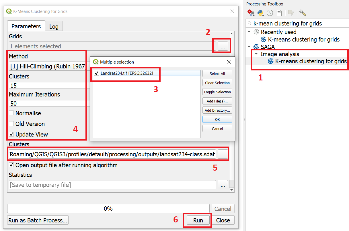
Fig. 5.11 Unsupervised classification using the ‘K-Means clustering’ tool
- Task 10
Repeat the Unsupervised classification for the ‘ASTER123N’ and the ‘Landsat234_+_ASTER123N’ stack. Name the resulting files as ASTER123N_class and Landsat234_ASTER123N_class, respectively.
You should now have three distinct Classifications.
5.4. Analysis
At this point, you have results of the unsupervised classification for three band stacks. Namely,
Landsat234_class - a mono-temporal and multi-spectral classification map, using Landsat bands from April 2010.
ASTER123N_class - a mono-temporal and multi-spectral classification map, using ASTER bands from June 2010.
Landsat234_ASTER123N_class - a multi-temporal and multi-spectral classification map, using bands from Lansat and ASTER for April and June 2010.
In this part of the exercise, we answer the question: Which of the ‘classification maps’ distinguishes better between classes of land cover?
5.4.1. Calculating Basic Statistics
Zonal statistics will help us to know what is the predominant pixel value (i.e. class) within for a specific area. We will use the polygons in the ‘evaluation’ layer to compute zonal statistics and find out the predominant class for each polygon.
- Task 11
From the Processing toolbox, open the Zonal Statistics tool. Compute zonal statistics for each of the classification maps. For Statistics to calculate select only
majority. Type a meaningful and distinct prefix in Output column prefix each time. See Fig. 5.12 The tool will create columns with names that start with such prefixes.
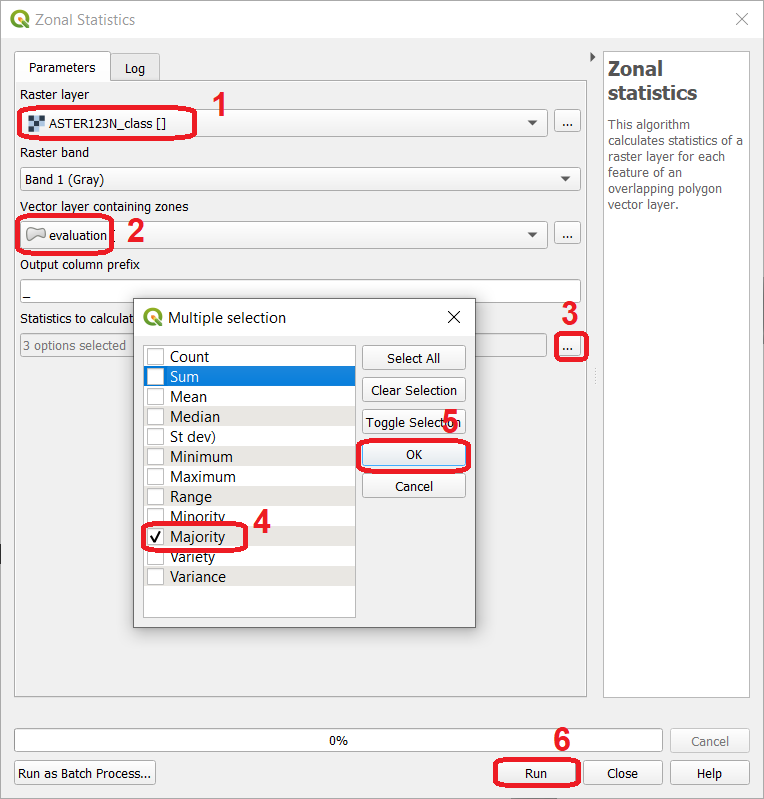
Fig. 5.12 Computing zonal statistics for the classification maps
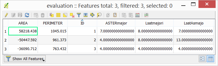
The statistics (majority) should now be in the attribute table of the ‘evaluation’ layer:
5.4.2. Comparison of Classification Results
- Task 12
Open the attribute of the ‘evaluation’ layer and examine the columns containing the result of zonal statistics. Remember, that such columns show the predominant class for each evaluation polygon (e.i., the class with more pixels inside each polygon) and each polygon in the ‘evaluation’ layer represent a distinct class of land cover.
Write in the table below, the total number of distinct classes that were identified in each classification map.
Classification Map
Number distinct Classes
Landsat234_class
ASTER123N_class
Landsat234_ASTER123N_class
Attention
Question. Which ‘classification map’ provided a better separation between classes? Why?
Section author: Zoltán Vekerdy, André Mano & Manuel Garcia Alvarez