9. Visualisation¶

9.1. Cartographic Grammar¶

The cartographic grammar defines a set of ‘rules of thumb’ for the Visualization of spatial data and the correct representation of spatial and temporal information on a Map. Cartographic grammar ensures that maps effectively communicate information to the map user.

For a more detailed explanation on Cartographic Grammar, visit https://kartoweb.itc.nl/TMT The Thematic Map Tutor will help you to understand which visual variable to use depending on the type of data you want to visualise. This will help you in completing the tasks below.

Attention

Question. Assume you were asked to make a map using following data:

What is the measurement level of the data?
Which visual variable(s) is (are) suitable to depict this data?
Which type of thematic map would you use to depict this data?

Task 1

Suppose you have to design symbols for a small scale (\(1:100.000\)) geological map. The following rock types have to be represented on the map:

igneous rock
metamorphic rock
consolidated sedimentary rock
unconsolidated sedimentary rock

You also have to map the terrain morphology, according to the following classification:

relatively flat terrain (slopes 0-7%)
rolling to hilly terrain (slopes 7-30%)
steep, rugged terrain (slopes > 30%)

All possible combinations of rock type and terrain classes may occur. Describe how you would set up this map: you do not have to draw the map or legend symbols, instead, describe:

which layer(s) of information you would put in the map and what visual variable(s) should be used to combine those layer(s) in a single map,
which legend titles and categories you would use, and
which type of map(s) to represent the data.

9.2. Critical Map Viewing¶

With the knowledge, you gathered in the previous section on Cartographic Grammar; you can critically look at existing maps and identify their shortcomings.

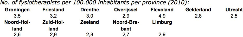
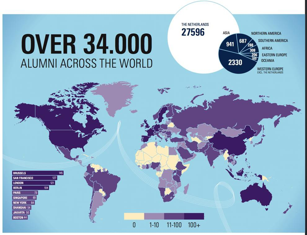
Task 2: Look carefully at the two maps below and use what you have learned about depicting quantitative data to analyse them critically.

Attention

Question.

What are some of the shortcomings these two maps above?

How will you solve such shortcomings? Give some examples.

Task 3: Before the next session in the Virtual Classroom, find a map (in the newspapers, on the web, in a research paper or a book) that you find interesting. You may select a map because you think something is wrong with it, but also because you particularly like it or think it is a well-made map.

Attention

Question.

What is interesting about the map you find in the previous task?
Can you give a summary of its flaws and strengths?

9.3. Creating a Topographic Map¶

In this section, you will create a small scale topographic map of a part of Switzerland, including the depiction of the 3D terrain using hill shading and layer tints.

Here, you will follow the “search, try & learn” principle. That means that we do not show you how to do things. Instead, we ask you to accomplish specific tasks and provide you with relevant information that will help you to achieve the tasks. The software skills necessary for this exercise were covered in previous sections.

In this exercise, you have to focus on the production of a cartographically well-designed map. It will be your responsibility to study the task carefully and search through the reference information for ideas and answers. With that knowledge, you have to decide which strategy to use to complete the task.

Important

Resources. You will require the latest LTR version of QGIS, plus the dataset visualization.zip.

9.3.1. Reference Material¶

Earlier exercises, using QGIS;
The QGIS training manual and the QGIS user guide.
The texts on Cartographic Visualisation in the Living Textbook;
The appendix on Shaded Terrain Models, which contains quick introductions to creating a shaded terrain model and other useful tools.

9.3.2. Understanding the Data¶

This is a detailed description of the datasets for creating a topographic map in this section.

Raster data

dem_90m.tif This is part of a Digital Elevation Model, produced by NASA from the Shuttle Radar Topography Mission (SRTM). During an 11–day mission in February of 2000, NASA obtained elevation data on a near-global scale to generate the most complete high-resolution digital topographic database of Earth. SRTM consisted of a specially modified radar system that flew onboard the Space Shuttle Endeavour. The data is freely available at http://www.jpl.nasa.gov/srtm.

Each cell has a value that represents the height in meters. The SRTM data was originally stored using geographical coordinates. However, this version is in meter coordinates in UTM zone 32N on the WGS84 datum (EPSG: 32632).

Vector data

All vector data was derived from the “EuroGlobalMap”, a Pan-European Database at Small Scale. It was an initiative from EuroGeographics, a cooperation of all European topographic services. The vector layers provided here are from version 7.0 (September 2013). The EGM Database is intended to be used in map scales of about \(1:1.000.000\). The EGM data was initially stored using geographical coordinates. However, this version is in meter coordinates in UTM zone 32N on the WGS84 datum (EPSG code 32632). EGM is open, and it can be downloaded from http://www.eurogeographics.org/products-and-services/euroglobalmap.

For this exercise, We have removed many of the attributes in the original datasets, and kept only small selection. A description of the attributes per dataset is given below:

builltUpArea.gpkg: NAMN1 = Name in German;
lakes.gpkg: NAMN1 = Name in German;
watercourse.gpkg: NAMN1 = Name in German;
railways.gpkg: TYPE: 31 = secondary, 33 = primary; TUNNEL: 0 = not in tunnel; 1 = in tunnel
ElevP.gpkg: Most important mountain tops and passes. Attributes NAMN1 = Name in German; ZV2 = height in meter above sea level;
towns.gpkg: NAMN1 = Name in German; PPL = population (in 2013);

The road data from EGM is notoriously incomplete and too general for the scale of the map that you will make. Therefore, we included data from the OpenStreetMap database. We extracted the road data for the categories that depict main roads. The OSM data was originally stored using geographical coordinates. However, this version is in meter coordinates in UTM zone 32N on the WGS84 datum (EPSG: 32632). Only a small selection of the original attributes of OSM was kept in this version. Those are:

osm_roads.gpkg: osm_id: unique id of each segment; type: motorway, primary, secondary, or trunk; tunnel: 0 = not in tunnel; 1 = in tunnel.

Note that the OSM data is very detailed. It is up to you to decide if you need all categories, or if it is better to delete or not show some of them. This will depend on the requirement of your user, and the choices of symbology that you make of this and the other data layers.

9.3.3. Map Making¶

Task 4

Open the QGIS project topographic_map.qgs. It contains all the layers you will need. Make a topographic map of this part of Switzerland (the “Berner Oberland”, highlands of Kanton Bern), that adheres to the following requirements:

The map shall present data in the information categories mentioned below. The visualisation shall be correct for the type of data, and it shall also be tailored for the specific combination. The required information categories are:
1. Terrain. The shape of the terrain shall be visualised using hill-shading in conjunction with layer tints. Consult the appendix Shaded Terrain Models to know how to create such a model. Refer to the theory in the Living Textbook and lecture slides to find examples of how to achieve such depiction. Give priority to the design of a sensible and readable visualisation. Something that gives the user a good impression of the shape of the mountains, in the country.
2. Infrastructure: roads and railways. The map shall show the number for the important roads.
3. Cities and towns. Place names shall be included for at least the larger cities.
4. Hydrography: lakes and rivers. The most important rivers and lakes shall show their names.
5. Optionally, the map shall include additional data that you gather from other sources (e.g., the Internet, atlases, and other). Useful additional information might be the names of mountain tops, the famous tourist sites, and others.
The map shall fit on an A4 landscape paper sheet. The outer bounds of the map shall be rectangular and match the extent of the DEM. The projection of the data shall be Universal Transverse Mercator (UTM) Zone 32N on the WGS84 datum. The data is already provided in that projection.
The map shall contain all necessary marginal information, such as title, legend, scale bar, etc.
The map shall be created for colour printing. The resulting map shall be exported as a PDF file. Use the Print Composer of QGIS to achieve this.

Important

This is a complex task! Please do not be satisfied too easily. Make tests of your results so far and study them critically. Ask family and friends, supervisors and your fellow students to give their opinion.

Attention

Question. Examining the topographic map you created in the previous task. What problems did you encounter during the map-making process?

Section author: Barend Köbben, André da Silva Mano & Manuel Garcia Alvarez