1. Spatial Data Models
1.1. Geographic Phenomena
 Geographic phenomena is a term for all phenomena with a spatial dimension, such as landcover or air pollution. Phenomena are geographic (spatial) when they:
Can be named or described;
Can be georeferenced (have a location on the Earth’s surface);
Can be assigned a time interval.
Geographic Phenomena can be divided into geographic objects and geographic fields, and Geographic Fields can represent geographic phenomena as discrete fields or continuous fields.
Attention
Question. Give some examples of phenomena for which one of the three elements above is missing. Can they be used in a GIS?
1.1.1. Objects and Fields
- Task 1
Complete the table below by indicating if the phenomenon on the left is an object or field and if it is discrete or continuous.
Phenomena
Field of Object
Discrete or Continuous
Wind direction
Temperature
Roads
Buildings
Field sample points
Landuse
Soil Type
1.1.2. Object’s Parameters
- Task 2
Which locational parameters can be used to describe objects? Not all the parameters that you identified are essential for all objects. Which of the locational parameters are important for the objects below?
Object
Parameter 1
Parameter 2
Parameter 3
Parameter n
House
Road
Well
Lakes
Rivers
1.1.3. Crispy and Fuzzy Boundaries
Another notion that is important for describing Geographic Phenomena is boundaries. We distinguish two types of boundaries: Crisp and Fuzzy.
Attention
Question. Can you give one example of a crisp boundary and one of a fuzzy boundary for any geographic phenomena?
1.1.4. Autocorrelation
There is one more concept that requires an introduction at this point, and that is Spatial autocorrelation. Spatial autocorrelation is based on Tobler’s first law of geography.
- Task 3
Define in your own words what spatial autocorrelation is.
Although all computer representations store data as finite representations, it is important that you realise that some phenomena show autocorrelation.
1.2. Computer Representations
The previous tasks did not use any software. This should not have surprised you because the focus, so far, was on understanding geographic phenomena and their characteristics. In this section, we will focus on showing how computers represent geographic phenomena. A good understanding of geographic phenomena will help you in choosing a suitable computer representation.
Here, you will explore different types of computer representations for geographic phenomena available in a GIS, and how to select the most suitable computer representation for a specific phenomenon. To get an overview of the different ways we can store geographic phenomena in a GIS, we are going to use the concept map of your Living textbook.
Attention
Question. Look for the term “Geographical Representation” in the Living textbook, and explore all related concepts two links apart. How many different types of representations of spatial data did you find?
Important
Resources You will require the latest LTR version of LTR version of QGIS, plus the dataset data_modeling.zip. When you unzip the dataset, you will find the following files inside:
Cities.csv– a comma-separated values file with city names;Spatial_data_modelling.qgs– A QGIS project preloaded with datasetselevation.tif– a digital elevation model;points.gpkg– a vector dataset representing elevation points.
1.2.1. Tesselations
Tessellations are a way to represent geographic phenomena in a GIS. A tessellation splits the geographic space into small cells in such a way that the complete area is covered by them. They are like tiles on a floor or a wall. In most cases, such tiles are square cells, and when all cells are equal in size, we call this a regular tessellation.
In a Regular tesselation, all cell have the same size and each cell is associated with a value (cell value). This value has a data type, such as integer or floating-point.
An integer data type is a number that does not contain any decimals. They are often used to indicate codes in a discrete field (e.g. a land use class). A float or floating-point data type is a number that may contain decimals. A floating-point data type that can store very big numbers (64bit) is known to have ‘double precision’, and it is often called “Double”. The table below shows a list of very common data types used in a GIS.
SHORT INTEGER |
Numeric values without decimals within a specific range. Application: store coded values. |
LONG INTEGER |
Numeric values without decimals within a specific range. The range is larger than a short integer. |
FLOAT |
Numeric values with decimals within a specific range. Single precision (32bits). |
DOUBLE |
Numeric values with decimal within a specific range. Double precision (64bits). |
TEXT |
Names or other textual qualities. |
DATE |
Dates and times. |
- Task 4
What data type would you use to represent a discrete field when you store it as a tessellation? And for a continuous field?
- Task 5
Boundaries in raster layers are both artificial and fixed. This has advantages and disadvantages. Can you give some examples of the advantages and disadvantages of artificial and fixed boundaries in raster layers?
- Task 6
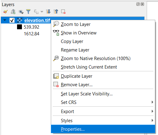
Open the ‘spatial_data_modelling’ QGIS project we provided in the dataset, and explore the properties of the tessellation representing elevation (
elevation.tif).How many rows/columns do the elevation.tif data has? Are the values of type integer or floating-point? What are the minimum and maximum values?
Hint: from the layers panel, right-click on the layer to access its Properties…. Once in the properties dialog, look into the Information dialog.
Attention
Question. What is the difference between a raster and a grid?
There are also Irregular tesselations. In irregular tessellations a geographic area is partitioned into cells which are not equal in size.
Attention
Question. It is often stated that irregular tessellations are more adaptive compared to regular tessellations. What exactly is meant by this?
- Task 7
Although there are multiple examples of irregular tessellations, you only have to study one example: “the Quadtree”. If you are not familiar with Quadtrees yet, refer to your Living Textbook for more information. The best way to learn how Quadtrees work is to construct one manually.
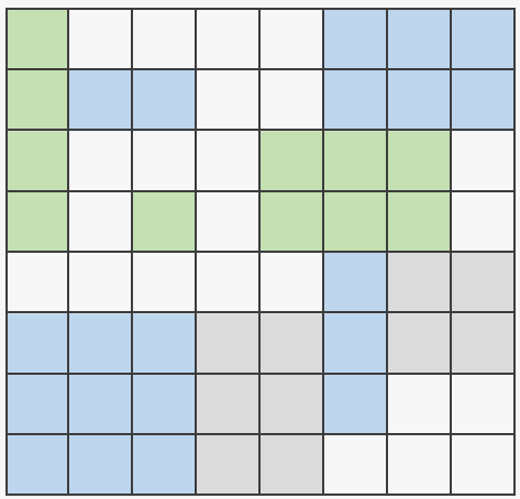
Construct the Quadtree for the raster layer shown below.
Attention
Question. Using a Quadtree to represent a geographic phenomenon improves computation performance (computations are faster). Do you understand how this works?
- Task 8
Calculate the area of the green, blue and white cells in the Quadtree in each level of the Quadtree. Assume the size of each original cell is \(100 \times 100 \ m\).
1.2.2. Vector Data Model
The main difference between our first data model (tessellation) and the vector data model is that tessellations do not explicitly store the georeference of the phenomena, but the vector data model does. This means that with every feature, coordinates are stored. In this section, we will discuss four examples of vector data representations: Triangulated Irregular Networks (TIN), Polygons, Lines and Points.
We start with the Triangulated Irregular Networks. (TINs) because they have some characteristics in common with tessellations.
Attention
Question. Which characteristics have in common TINs and tessellations?
- Task 9
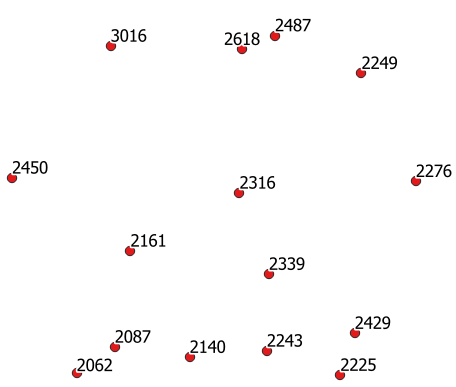
Using the picture below, manually create a TIN from the given points.
Attention
Question. You may be surprised, but not all triangulations are equally good. The standard triangulation is a Delaunay triangulation. Was your triangulation Delaunay?
- Task 10
In your QGIS project, you find a layer with points. Generate a Delaunay triangulation and compare the result with the tessellation you made.
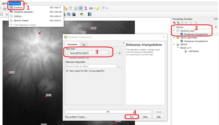
Fig. 1.1 Steps to create a Delaunay triangulation in QGIS
A triangulation can also be used to generate a continuous tessellated surface by means of interpolation. In those cases, each cell is assigned the value that is related to how far that cell is from the anchor points.
- Task 11
Create a tessellation using the TIN interpolation tool; use as input the anchor points you have in your QGIS project. Then, use the Identify tool to inspect the cell values.
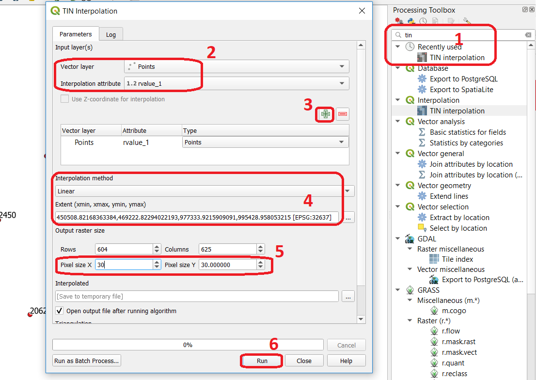
Fig. 1.2 Steps to create a tessellation from a TIN in QGIS
Important
QGIS. QGIS does not perform ‘on the fly interpolation’ – meaning that any point you click within your interpolated surface will have its value calculated on the spot. Instead, what QGIS does is to generate a tessellation of predefined cell size where each cell as a fixed value. ‘On the fly’ interpolations are supported in ArcGIS, for example; however, it is a functionality that will only exist within ArcGIS – the resulting data structure cannot be exported and used in other software packages.
Attention
Question. What exactly are the advantages of a TIN over a tessellation?
- Task 12
In your data, you find a table
Cities2.csv. Try to use this table to create a point layer in QGIS. Start a new QGIS project and add the layer to QGIS using the Delimited Text option.
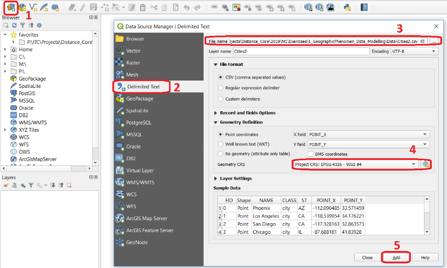
Fig. 1.3 Steps to create a point layer using a CSV file in QGIS
From the previous task, you should have clear that points are the simplest of geometries – they have a Y and X coordinates that anchors them to the spatial frame you are working on.
Another way of representing geographic phenomenon in the vector data model is using a Line representation. A line is nothing more than two or more connected points.
Attention
Question. What is the difference between nodes and vertices, and how can we know the direction of a line?
The last representation in the vector data model is polygons. Polygons are one of the most well-known and commonly used vector data models. There are two important parts when using a polygon data model: the boundary model and the Topological model.
The boundary model explains how areas are represented and by storing the closed boundary that defines an area. A closed boundary is defined by a closed line (consisting of nodes and vertices, where the start and end vertices intersect). When representing the footprints of houses or the borders between countries, the boundary of each feature (house/country) is stored individually.
The Topological model is discussed in the the following section on Topology.
- Task 13
Read the section
Area representation and describe in your own words the problems that may arise when using the boundary model without topology.
1.2.3. Topology
The third topic in this exercise is Topology. You will first have to understand what topology is before learning different ways to use it. Topological properties are geometric properties and spatial relations that are not affected by the continuous change of shape and size of a vector data layer (points, lines, or polygons).
- Task 14
Imagine you are looking at a map (take any map you like). Make a small list containing at least five examples of spatial topology that are visible in your map and five examples of properties that are not topological (use the table below).
Example
Topological
Non-topological
1
2
3
4
5
When looking at two polygons, we can define all their possible topological relationships. To do so, we must describe each polygon in terms of its boundary and its interior (the area inside the boundary). Read Topological relationship.
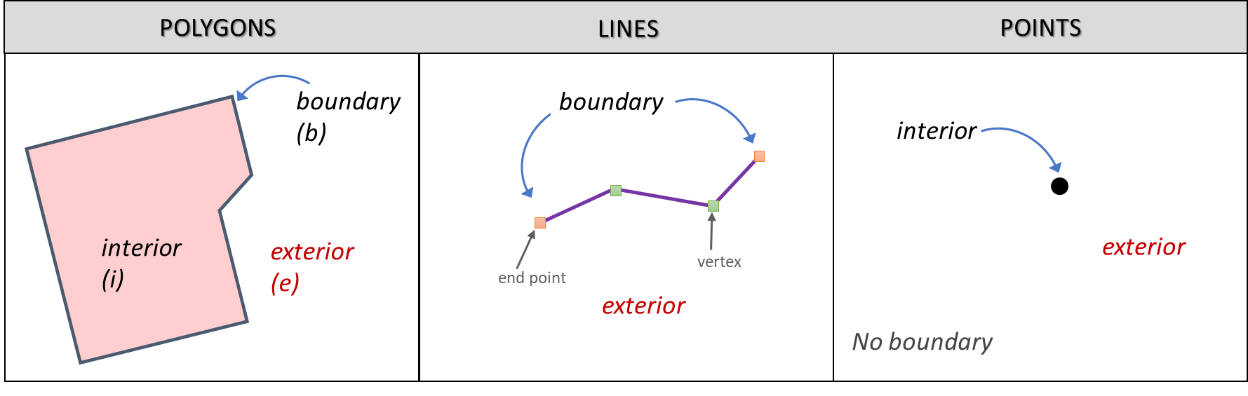
Fig. 1.4 The boundary, interior and exterior of polygons, lines and points
Attention
Question. What is the correct mathematical (set theory) expression that describes the covers relationship? How does this expression differ from the covered by relationship?
By now, you should understand what topology is, but you may wonder how it can be used. During the coming exercises, you will see many different uses, but for now, focus on an example given in the Topological data model.
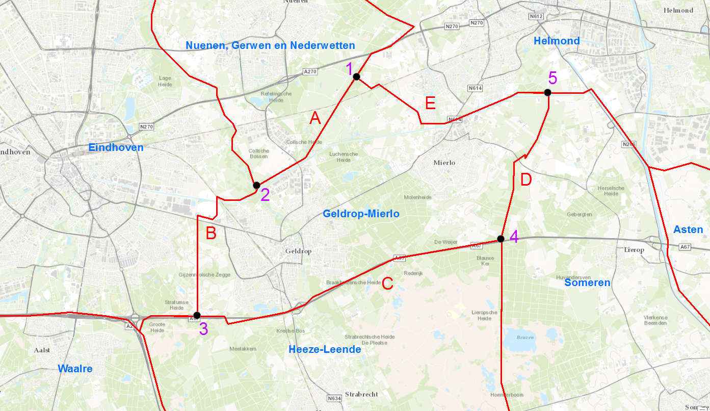
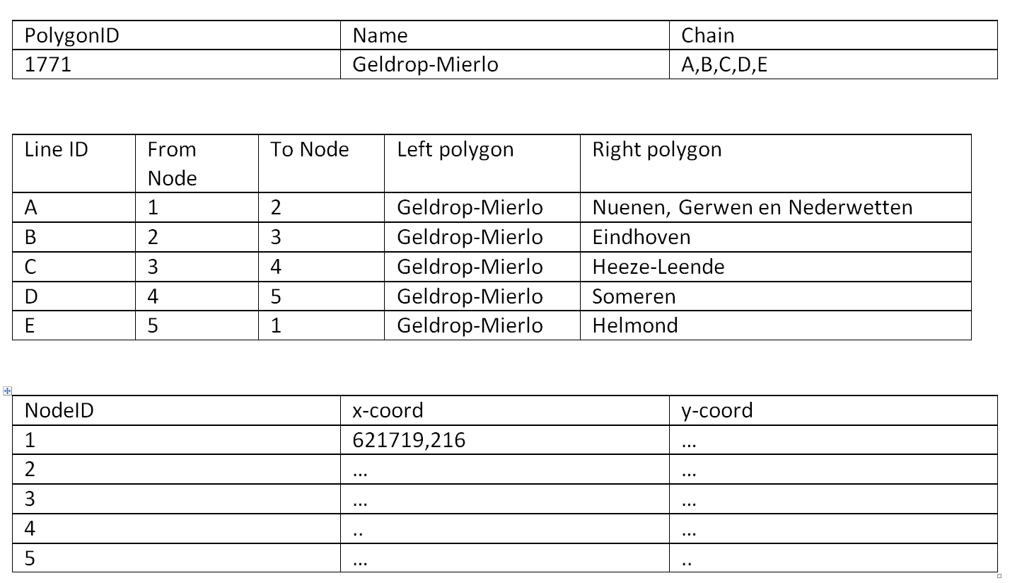
Attention
Question. For the map below, can you complete its corresponding attribute table following the topological data structure? The map below shows a polygon layer based on administrative units (municipalities). Focus your attention on the Geldrop-Mierlo municipality and its adjacent municipalities. The table below shows an example of the topological data structure for Geldrop-Mierlo.
Topology can also be used to ensure consistency of the geometries in a vector layer. There are five rules of Topological consistency, which you should know about.
- Task 15
Identify for every example below which rule of topological consistency is violated.
Example
Rule(s)
The boundary of a polygon is not closed.
Two lines cross each other without an intersection.
There is a gap between two polygons.
Two polygons overlap.
Additional uses of topology will be discussed in the sections: Data Entry, Using Spatial SQL and Networks. In this course, you only need to understanding Topology in a conceptual level.
Attention
Question. The following statements are made about time. What is your opinion on them? Are they true or false?
1.2.4. Temporal Dimension
In many situations, it is not enough to describe geographic phenomena only in terms of space, but also in terms of time because such phenomena change over time. The change may be relatively fast (like the clouds in the sky, hurricanes, and traffic) or slow (like the movement of a glacier).
To including time in the representation of spatial data, we talk about the Spatial-temporal data model. This model defines different types of change: change in attributes, change in location (movement) and change in shape (growth) or combinations of these three.
- Task 16
Below you see a list of different types of change and some combinations. Can you write down an example for each type?
Type of Change
Examples
Attribute
Attribute and Location
Attribute and Shape
Location
Location and Shape
Attribute, Location and Shape
Attention
Question. The following statements are made about time. What is your opinion on them? Are they true or false?
Although time is continuous in nature, in a GIS it is always represented in a discrete manner.
There are many examples of spatial phenomena for which valid time is simply unknown.
Branching time should be looked at into the future, as the past is already known and has only one branch.
Time granularity is comparable to the spatial concept of resolution.
Note
Reflection.
So far, you used vector representation of area features stored as Shapefiles. Are these shapefiles storing topology? In other words, do Shapefiles use a topological data model?
In this exercise, we have mainly focussed on 2-D data modelling examples. Yet, the real world is 3D. Do you know any examples in which a real 3-D data model would be needed? Is there also a 3-D topology?
Which other compression techniques exist besides Quadtrees?
Besides rectangular cells, other shapes can be used. What are the advantages of using Hexagonal cells?
Make a comparison between raster and vector data models and list the advantages and disadvantages of each one.
Section author: Ellen-Wien Augustijn, André da Silva Mano, Manuel Garcia Alvarez & Amy Corbin